
LLM from Scratch (TinyLLaMA)
Published:
- Introduction
- Tokenization: From Text to Tokens
- Embeddings: From Tokens to Vectors
- Attention: Where Magic Happens
- KVCache: Save What have been Computed
- Multi-head Attention: Learn Different Rules of Language
- RoPE: Learn Distance between Tokens
Introduction
I’ve been wanting to learn about the LLM for quite a long time, but didn’t have the time to do so until now. So, I decided to implement a simple LLM using my way of learning, which is to implement it from scratch.
Ground Rules
I have set some ground rules for myself to follow while implementing the LLM:
- No wheels: I will implement everything (except basic ops like
matmul) from scratch. - Actual LLM: I will aim to implement inference loop for TinyLLaMA, an actual LLM.
- Understand math, not code: I will study the math behind the LLM.
Tokenization: From Text to Tokens
Languages like English are formed from basic semantic units – words. For LLMs to understand and process language, we also need to define a set of basic semantic units – LLM’s vocabulary. An intuitive choice for these units would be directly using words. However, this approach has an obvious problem: LLMs wouldn’t be able to recognize any word that is not in its vocabulary, such as phishy. To solve this problem, LLMs like TinyLLaMA use a more delicate algorithm named Byte Pair Encoding (BPE) to tokenize words into subword units.
The idea behind BPE is that if certain subword units appear adjacent to each other frequently, then they are likely to be semantically related and thereby can be merged.
Suppose we have the following sentence.
FloydHub is the fastest way to build, train and deploy deep learning models. Build deep learning models in the cloud. Train deep learning models.
BPE will start from the most basic unit – letters, and gradually merge adjacent units that appear frequently together. So, in the beginning, BPE compute the frequency of each adjacent pair of letters, yielding the following table.
| Key | Count | Key | Count | Key | Count |
|---|---|---|---|---|---|
| de | 7 | in | 6 | ep | 4 |
| lo | 3 | ee | 3 | le | 3 |
| ea | 3 | ar | 3 | rn | 3 |
| ni | 3 | ng | 3 | mo | 3 |
| od | 3 | el | 3 | ls | 3 |
So, we can merge the most frequent pair de, treat it as a single unit, and represent it as X. Then we get the following sentence.
FloydHub is the fastest way to build, train and Xploy Xep learning moXls. Build Xep learning moXls in the cloud. Train Xep learning moXls.
Then we can repeat the same process, merging the most frequent pair into new units, until we have reached a preferred vocabulary size \(N\). In particular, if we don’t set a limit on the vocabulary size, we can keep merging until every unit is a word again, which is the case of using words as tokens.
Why this makes sense?
Though beginning with cruel statistics, BPE can effectively capture the semantic relationship between subword units. For example, in the above sentence, tion appeared in construction, location, and ...tion has the same semantic meaning of being a noun suffix. So, if there are sufficiently many words that share the same suffix, BPE will eventually merge the suffix into a single unit, which can be easily recognized by the LLM as a noun suffix.
As TinyLLaMA is trained on a large corpus of text, we are unable to reproduce its tokenization process. We thereby reuse autotokenizer from HuggingFace to tokenize the input text into tokens.
tokenizer = AutoTokenizer.from_pretrained("TinyLlama/TinyLlama-1.1B-Chat-v1.0", cache_dir="./")
print("--- Test Tokenizer ---")
tokenized = tokenizer("Hello, World!")
tokens, mask = tokenized["input_ids"], tokenized["attention_mask"]
print(f"Hello World! ===> {tokens}")
Embeddings: From Tokens to Vectors
In the language we use from day to day, we have letters, words. In the world of AI models, however, we only have numbers and vectors. So, for LLMs to understand and process language, we need to convert words into numbers. This is where embeddings come in; it is essentially a function that maps tokens to vectors. For example, we can have a function \(f\) that maps the token Love to a numerical vector.
Note that the embedding function is not simply giving every token a random vector. Instead, it is designed to capture the semantic relationship between tokens. The following figure illustrates this idea; the word France is mapped to a vector that is close to the vector of Paris, while Germany is mapped to a vector that is close to Berlin. This way, the LLM can understand the semantic relationship between these words through their embeddings.

Attention: Where Magic Happens
Attention is the core component of LLMs. It puts three vectors – \(Q\), \(K\) and \(V\) – into each token; their semantic meaning is as follows:
Query (\(Q\)): It represents the token’s query vector, which represents the token’s query for information from other tokens.
Key (\(K\)): It represents the token’s key vector, which, receives a query \(Q\) and respond how well \(Q\) and itself \(K\) relates.
Value (\(V\)): It represents the token’s value vector, which represents the actual contextual information of the token.
To obtain these three vectors, LLMs maintain three trainable weight matrices – \(W_Q\), \(W_K\) and \(W_V\); multiplying token’s embedding with these weight matrices gives us \(Q,K,V\).
\[Q = XW_Q^T, \quad K = XW_K^T, \quad V = XW_V^T\]Why not \(W_Q x\)?
This is because we want to maintain row-major order for token’s embedding \(X\), whose shape is
[T, H]. \(T\) is the number of tokens, and \(H\) is the embedding dimension. Such row-major order is more cache-friendly as computers store data in a row-major order, i.e., a row \([x_1, x_2, x_3]\) located in neighboring addresses with better spatial locality while column \([x_1, x_2, x_3]^T\) is not.
After we have \(Q,K,V\), we now can do the famous attention equation:
\[\text{Attention}(X) = \text{softmax}(\frac{QK^T}{\sqrt{d}})V\]Let’s first look at \(QK^T\), it essentially computes the inner product of each \(q_i=x_iW_Q^T\) and \(k_j=x_jW_K^T\). By easy linear algebra, \(q_i\cdot k_j^T\) equals to \(x_iW_Q^TW_Kx_j^T\), which is a inner product between \(x_i\) and \(x_j\) as we’re working with row-major vectors.
Inner product’s definition \(x\cdot y = \|x\|\|y\|cos\theta\). When both \(x\) and \(y\) are unit vectors, the inner product is simply the cosine similarity between these vectors. Attention score is also a similarity score between tokens, with additional information from the weight matrices \(W_Q\) and \(W_K\).
The normalization term \(\sqrt{d}\) is to debloat the attention score. Assume \(q,k\sim N(0,1)\), the variation of \(q\cdot k^T\) is \(\sum_i^d Var(q_ik_i) = \sum_i^d Var(q_i)*Var(k_i) = \sum_i^d 1 = d\), so dividing by \(\sqrt{d}\) is equivalent to normalizing the variation of attention score to 1, which prevents \(\text{softmax}\) from being oversaturated (due to dimension increase) and thereby having vanishing gradients.
Saturated softmax means that if the input to softmax is out of a reasonable range, e.g., \(\text{softmax}(x\geq 5)\cong 1\). If all components of the input vector, due to dimension increase, are larger than 5, then the output of softmax will all be near a constant 1, which causes the gradient to vanish (near 0) as constant has zero gradient.
KVCache: Save What have been Computed
In attention computation, we need to compute \(K,Q,V\).
Multi-head Attention: Learn Different Rules of Language
The above mentioned attention is also called single-head attention, as it only has one set of weight matrices \(W_Q\), \(W_K\) and \(W_V\). However, in real-world languages, there are different rules that govern the relationship between tokens, such as semantics, syntax, and so on. These rules might be very different from each other, so maintaining only one weight matrix causes training to be difficult as models might struggle to learn different rules back and forth with different batches of training data.
The idea behind Multi-head Attention (MHA) is simple, we partition weight matrices \(W_*\) into smaller matrices \(W_*^i\) and let them to interact with \(x\) separately, learning different rules of language in different heads.
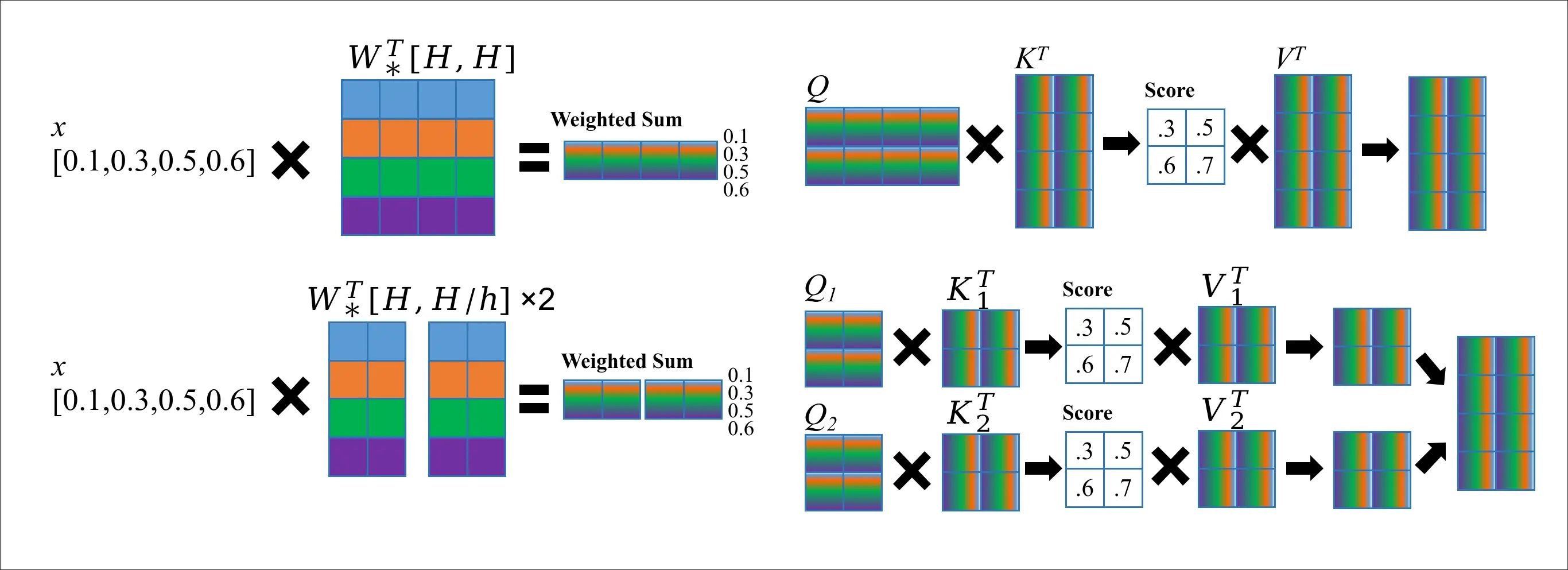
I found it’s simpler to directly understanding the MHA by looking at the shapes of the matrices. Assuming we have number of tokens \(T\), dimension of embedding \(H\), then the shape of \(Q,K,V\) would be \([T,H]\). So, if we want to split them into \(h\) heads, then the shape of each \(Q^i,K^i,V^i\) would be \([T,H/h]\). We treat these \(Q^i,K^i,V^i\) as usual and plug them into the attention equation,
\[\text{Attention}(X^i) = \text{softmax}(\frac{Q^i{K^i}^T}{\sqrt{d_i}})V^i\]We then have \(\text{Attention}(X^i)\) with shape \([T,H/h]\), which can be concatenated together back to a matrix of shape \([T,H]\), which is the result of MHA.
How this works? Let’s see the following picture. On the left, we can see MHA actually doesn’t change the calculation of \(Q,K,V\); we just split them afterwards. On the right, we can see that the MHA calculates attention using split \(Q^i,K^i,V^i\). Though this might seem trivial, this actually separate the gradient of different heads as they are simply concatenated. This allows the different part of \(W_*\) (i.e., \(W[H,0{:}H/h]\) and \(W[H,H/h{:}H]\)) to learn different patterns of the language when doing backpropagation.
Variant: Grouped Query Attention
RoPE: Learn Distance between Tokens
Note that the current form of attention is permutation invariant, which means that the attention score between two tokens is not affected by their relative position. This is a problem as the meaning of a sentence is often determined by the order of words. Therefore, we hope to have a way of injecting positional information into the attention mechanism.
Clearly, in human language, the relative position between tokens is more important than their absolute position. Knowing a word in the \(X_{\text{th}}\) position of a sentence doesn’t tell us much, but knowing that a word is right after am/is/are can be very informative. Therefore, we want to have a way of encoding the relative position between tokens into the attention mechanism.
To encoding the relative position between tokens, we can define a linear transformation \(R_mx_m\), where \(x\) is a token and \(m\) is its absolute position index.
What are we doing here? We wish to encoding the relative position between token \(m\) and every other tokens \(0,1,..m-1,m+1,..L_{max}\) into the components \([x_m^1,x_m^2,..,x_m^H]\) of token vector \(x_m\).
We wish we have the following property for this function:
\[{R_mx_m}^TR_nx_n = g(x_m,x_n,m-n),\quad R_0=I\]This property means that the inner product between two tokens’ positional embeddings can be expressed as a function of their relative position \(m-n\). This way, the attention score between two tokens can be influenced by their relative position. Particularly, we define \(R_0=I\) for convenience. Moreover, we also want to have \(R_m\) doesn’t modify vector’s length, i.e., \(\|R_mx_m\|=\|x_m\|\). Because, the following equation holds:
\[m=n\Rightarrow (R_mx_m)^T(R_mx_m) = g(x_m,x_m,0) = (R_0x_m)^T(R_0x_m)\Rightarrow \|R_mx_m\|=\|x_m\|\]As \(R\) maintains length, it can only be a composition of rotation and reflection. Formally, by polarization identity, we can derive \(R_m\) keep the inner product between any two vectors, i.e., \(x^TR_m^TR_my = x^Ty\). So, we can further derive that \(R_m^TR_m = I\), which means \(R_m^T = R_m^{-1}\).
So, in the end, we have:
- \(R_0=I\), manually define position \(0\) provides no information
- \(R_m\) is orthogonal matrix, \(R_m^T=R_m^{-1}\)
- \(R_m\) keeps length, \(\|R_mx\|=\|x\|\)
This naturally leads us to the idea of using rotation as the linear transformation.
Rotation in Higher Dimension
It might seem unintuitive to use rotation in higher dimension, but it’s actually quite simple. A high-dimensional rotation matrix (Givens rotation in n-dimensions, rotating in the i-j plane):
\[R(i, j, \theta) = \begin{bmatrix} 1 & & & & & \\ & & \ddots & & & \\ & & \cos\theta & -\sin\theta & & \\ & & \sin\theta & \cos\theta & & \\ & & & \ddots & & \\ & & & & & 1 \end{bmatrix}\]We can choose a pair of adjacent dimensions (i.e., \(\|i-j\|=1\)), and rotate around these two dimensions. By repeating this process with multiple different planes for sufficiently many times, we can obtain any arbitrary rotation. In this way, we end up with this block-diagonal rotation matrix for RoPE:
\[R_m = \begin{bmatrix} \cos m\theta_0 & -\sin m\theta_0 & 0 & 0 & \cdots & 0 & 0 \\ \sin m\theta_0 & \cos m\theta_0 & 0 & 0 & \cdots & 0 & 0 \\ 0 & 0 & \cos m\theta_1 & -\sin m\theta_1 & \cdots & 0 & 0 \\ 0 & 0 & \sin m\theta_1 & \cos m\theta_1 & \cdots & 0 & 0 \\ \vdots & \vdots & \vdots & \vdots & \ddots & \vdots & \vdots \\ 0 & 0 & 0 & 0 & \cdots & \cos m\theta_{d/2-1} & -\sin m\theta_{d/2-1} \\ 0 & 0 & 0 & 0 & \cdots & \sin m\theta_{d/2-1} & \cos m\theta_{d/2-1} \end{bmatrix}\]Decision of Rotation Angle
The last question is, if \(R_m\) is a rotation matrix, how do we decide the rotation angle \(\theta_i\). Let’s try a few naive solutions.
- Constant angle: \(\theta_i=\theta\)
If \(\theta\) is small (low frequency), then the rotation is very slow, words that are close to each other (e.g., \(2\theta\) and \(\theta\)) might be hard to distinguish. If \(\theta\) is large (high frequency), then the rotation is very fast, far-away word (e.g., \(1000\theta\)) would be random (many round of \(2\pi\)).
- Linear formation: \(\theta_i=(2i\pi)/L_{max}\) where \(L_{max}\) is the maximum sequence length.
The problem here is that linear formation doesn’t cover sufficiently large frequency space. \(L_{max}\) could be very large (>128K), but the maximum dimension is more bounded (~2048). Therefore, this formation creates a very dense frequency space, where \(\theta_{10}=0.0005\) and \(\theta{100}=0.005\) does make much differences.
Why linear formation don’t work? Recall that we’re trying to encode the relative position between \(x_m\) with every other tokens \(x_0,x_1,..,x_{m-1},x_{m+1},..x_{L_{max}}\), which is \(L_{max}-1\)’s distance. But our token vector only has \(d=H\) components. Any linear mapping from \(L_{max}\) to \(d/2\) will result in a very dense projection, which means that many different relative positions will be projected to very close angles, making them hard to distinguish.
So, it would be straightforward to use a exponential formation and allow \(\theta_i\) to grow sparsely across the frequency space to capture all \(L_{max}-1\) distances, i.e., \(\theta_i=N^{-2i/d}\). The \(2/d\) factor is to get a dimension-invariant angle. The negative sign is to make sure the angle is exponentially decreasing, otherwise it will just explode. (PS: we can make \(\theta_0=2\pi\), but it won’t be that useful). As for \(N\), it can be decided based on \(L_{max}\), the longer the sequence is, the more sparse the frequency space is, so we can choose a larger \(N\). In TinyLLaMA, \(N=10000\).
Exponential formation creates a sparse frequency space, and covers a wide range of frequencies. Thereby, close words can be distinguished by low-frequency rotations with smaller \(i\) while far-away words can be distinguished by high-frequency rotations with larger \(i\).
| i | \(\theta_i\) |
|---|---|
| 0 | 1 |
| 10 | 0.91 |
| 100 | 0.41 |
| 200 | 0.17 |
| 500 | 0.01 |
| 1000 | 0.0001 |